Package:
pdbmdauto1.2.9 · Template id:pdbmdauto-pipelineInstall the package from the Marketplace, then open this template from Start from Template. Its inputs ship with the package or are fetched for you — the walkthrough says which, and whether it needs the network.
The bundled template takes one PDB identifier and returns a complete, protonated, solvated and energy-relaxed system with a short test trajectory — every intermediate on disk.
| Structure | 4Z8J, 0.95 Å — the SNX27 PDZ domain bound to the C-terminal PDZ-binding motif of the parathyroid hormone receptor |
| Chains | A the PDZ domain (101 residues in sequence, 96 resolved) · B the peptide QEEWETVM (8, 7 resolved) |
| Unresolved residues | six, all N-terminal: A Gly33–Gly37 (GSHGG, a tag remnant) and B Gln586 |
| pH | 7 |
| Force field | amber99sb, TIP3P water |
| Box | 6.45 nm cube: the protein’s diameter plus 1.0 nm on every side |
| Ions | 0.15 M NaCl, neutralised — 25 Na⁺, 24 Cl⁻ |
| Production | 2 ps (1000 × 2 fs) at 300 K |
| Runtime | 3–5½ min on an Intel laptop (three runs), ≈ 2 min on an Apple Silicon Mac Mini, measured on 1.2.0, whose box was a smaller 5 nm cube; the first install adds 3½ min on a Mac, ≈ 20 min on Windows through WSL2 |
Before you run
- Network. Step 1 fetches 4Z8J from the RCSB PDB. Offline, set Input mode to a local file.
- A working directory. Everything lands under
<working directory>/pdbmdauto-e2e-full/e2e_4z8j/(the case name comes from the template). Choose an empty folder. - The first install builds a 3.1 GB environment once (GROMACS, ProMod3, OpenStructure, PDB2PQR, PROPKA, Biopython, OpenMM). On Windows Salpa sets that environment up inside WSL2 for you.
The structure
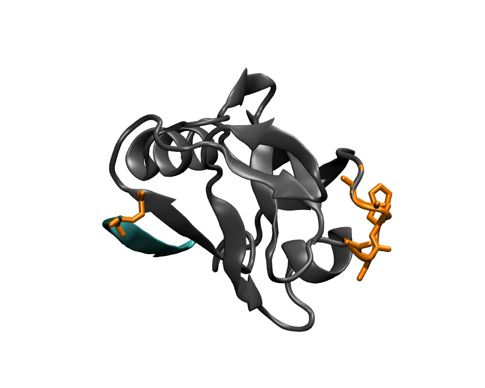
The model after step 5. The five-residue tag on the domain’s N-terminus and the peptide’s first residue were not located in the experiment; ProMod3 built them. They hang off the ends, where a terminal extension has nothing to pack against — a reminder that a rebuilt residue is a prediction.
The pipeline
Eleven nodes in a line. Each reads what the previous one wrote and adds its own files to the case
directory. Paths below are relative to pdbmdauto-e2e-full/e2e_4z8j/.
1 · PDB FASTA Parser — Biopython, RCSB PDB
| takes | the PDB id 4Z8J, pH 7, case name e2e_4z8j |
| writes | 4Z8J.pdb, 4Z8J_rcsb.fasta, chain_A.fasta, chain_B.fasta, missing_residues_chain_A.csv, missing_residues_chain_B.csv |
| set here | Input mode (PDB id or local file), PDB id, pH |
Downloads the entry, splits it by chain, and reads the header’s REMARK 465 records into one CSV
per chain: which residues the sequence has and the coordinates do not. For 4Z8J that is five rows
for chain A (33–37) and one for chain B (586).
2 · Generate Alignment
| takes | the structure and per-chain sequences |
| writes | A/homology.ali, B/homology.ali (+ .seq) |
Aligns each chain’s resolved residues to its full sequence — the gaps in that alignment are what step 5 will build.
3 · Multi-Chain Alignment
| writes | Merge/homology.ali |
Consolidates the per-chain alignments into one, so the complex is modelled as a unit.
4 · Merge PDB Chains — Biopython
| writes | Merge/merge.pdb, Merge/chain_type.json, Merge/chain_name.json |
Writes the selected chains as one model, dropping water and hetero residues (ligands, ions, cofactors). If your system needs a bound ligand, this is the step to notice.
5 · Fix Missing Residues — ProMod3 / OpenStructure
| takes | Merge/merge.pdb, Merge/homology.ali |
| writes | Merge/alignment_A.fasta, Merge/alignment_B.fasta, Merge/fixed.pdb |
Builds the six missing residues and reconstructs sidechains. It does not minimise: ProMod3’s own
minimisation is left out, and step 6 minimises the model in vacuo. In the reference run
chain A went from 96 to 101 residues and chain B from 7 to 8. Two things to know: ProMod3
renumbers from 1 (merge.pdb carried 38–133 and 587–593; fixed.pdb reads 1–101 and 1–8),
and the Model Terminal Extensions option has no effect in this version — termini are always
built.
6 · pKa + GROMACS EM — PROPKA, PDB2PQR, GROMACS
| takes | Merge/fixed.pdb, pH 7 |
| writes | gmx/propka.pqr, gmx/protonated.pdb, gmx/pdb2gmx.gro, gmx/pdb2gmx.top (+ per-chain .itp, posre.itp), gmx/box.gro, gmx/em_noconstr.*, gmx/em_hbonds.* |
| set here | force field and water model (amber99sb, tip3p), the two .mdp files |
pdb2pqr --ff AMBER --titration-state-method=propka --with-ph=7.00 decides which His, Asp, Glu,
Lys and Arg are charged at pH 7 and adds hydrogens; pdb2gmx -ff amber99sb -water tip3p -ignh
writes the topology; editconf -d 2 puts a box around it; two steepest-descent minimisations
follow, first without constraints, then with H-bond constraints. Reference run: the constrained
one converged to Fmax < 1000 in 15 steps at −1.26 × 10⁴ kJ/mol.
7 · Original Atom Groups — GROMACS
| writes | gmx/index.ndx with two extra groups, OriHeavy and OriBackBone |
Marks which atoms came from the experiment, so the next step can hold them still while the rebuilt
ones move. Which residues were rebuilt comes from Merge/rebuilt_residues.json, written by step 5
in the model’s own numbering. Reference run: OriHeavy 780 atoms, OriBackBone 410. That is the
103 resolved residues: 101 × 4 backbone atoms, plus 3 for each of the two C-termini, whose oxygens
(OC1, OC2) are not backbone atoms. Exactly the six rebuilt residues are left out.
(Up to 1.2.5 this step matched deposited residue numbers against the renumbered model and got
776 and 414 with the wrong residues.)
8 · GMX MD Relaxation (restrained) — GROMACS, protocol full_4step
| takes | gmx/em_hbonds.gro, gmx/pdb2gmx.top, gmx/index.ndx |
| writes | gmx/nvt_fixOri.*, gmx/nvt_fixOriBackbone.*, gmx/mm1.*, gmx/mm2.* |
| set here | Protocol (full_4step here, em_only at step 10) |
Four stages in vacuo: 5 ps of NVT at 300 K with every experimental heavy atom frozen, the same with only the experimental backbone frozen, then two conjugate-gradient minimisations. The rebuilt residues settle; the crystal structure does not drift. Reference run: the last minimisation converged to Fmax < 100 in 7 steps at −1.55 × 10⁴ kJ/mol. This is the slowest step — 84 s on a cold laptop, 222 s on the same laptop once hot.
9 · GMX Solvate & Ionize — GROMACS
| takes | gmx/mm2.gro, gmx/pdb2gmx.top, demo_data/ions.mdp (shipped with the node) |
| writes | gmx/box.gro (rewritten as the padded cube), gmx/solv.gro, gmx/ion.tpr, gmx/ion.gro, gmx/topol.top |
| set here | box size (auto) and padding, salt concentration, ion names |
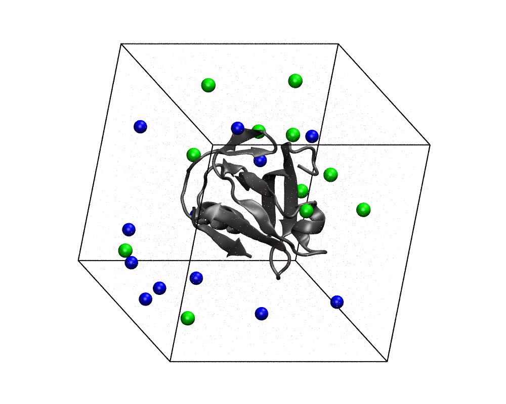
editconf -bt cubic -d 1.0 -c: a cube sized from the protein’s diameter plus 1.0 nm on every
side, so the protein stays 2 nm from its periodic images however it turns. Then solvate with
SPC216 and genion -neutral -conc 0.15 -pname NA -nname CL. Reference run: a 6.45 nm cube and
8,170 waters; the complex carried a charge of −1, so 25 Na⁺ and 24 Cl⁻ bring it to zero at 0.15 M;
26,202 atoms in total. The box follows the protein’s diameter after the relaxation before it,
which is molecular dynamics and does not repeat exactly, so these counts vary from run to run:
six runs on one Mac gave 25,866 to 27,724 atoms in a 6.41 to 6.56 nm cube.
10 · GMX MD Relaxation (solvated) — GROMACS, protocol em_only
| takes | gmx/ion.gro, gmx/topol.top |
| writes | gmx/em.tpr, gmx/em.gro, gmx/em.log, gmx/em.edr |
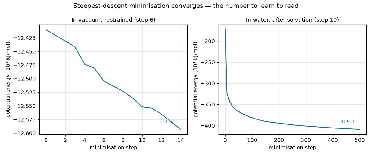
One steepest-descent minimisation of the whole box, 500 steps, tolerance 500. Reference run: it
stops at the step limit with Fmax ≈ 7.5 × 10³ kJ mol⁻¹ nm⁻¹ (on a glutamate’s carboxylate;
the largest remaining force changes from run to run) and a potential energy of −4.09 × 10⁵ kJ/mol — the water has relaxed onto the protein (compare the curve below) but the
tolerance is not met. For the demonstration that is enough; for a production study raise
nsteps in em.mdp until it converges.
11 · GROMACS MD Run (Local) — GROMACS
| takes | gmx/em.gro, gmx/topol.top, demo_data/md.mdp (shipped with the node) |
| writes | gmx/md.tpr, gmx/md.gro, gmx/md.trr, gmx/md.edr, gmx/md.log, gmx/md.cpt |
| set here | the .mdp file — steps, time step, thermostat |
1000 steps of 2 fs at 300 K (velocity rescaling, no pressure coupling), coordinates every 100 steps:
11 frames in md.trr (uncompressed; no .xtc is written). gen_seed = -1 in the shipped
md.mdp, so velocities — and therefore trajectories — differ from run to run. Reference run:
31.6 ns/day on the cold laptop, 9.1 ns/day once hot.
Looking at the result
In Salpa (0.9 or later), each step’s View tab draws the structures it wrote. Select the node and open View in the panel on the right, or right-click the node and choose View; View in window keeps the view open beside the workflow. A step opens on its main structure, and its Files menu lists the rest:
| Step | Opens on |
|---|---|
| 4 · Merge PDB Chains | Merge/merge.pdb |
| 5 · Fix Missing Residues | Merge/fixed.pdb |
| 6 · pKa + GROMACS EM | gmx/em_hbonds.gro; gmx/protonated.pdb and gmx/propka.pqr are under Named in results in Files |
| 8 · GMX MD Relaxation (restrained) | gmx/mm2.gro |
| 9 · GMX Solvate & Ionize | gmx/ion.gro |
| 10 · GMX MD Relaxation (solvated) | gmx/em.gro |
| 11 · GROMACS MD Run (Local) | gmx/md.gro; tick md.trr in Files and press Play (▶) for the eleven frames |
Outside the app, the same files:
vmd Merge/fixed.pdb                      # the completed model — colour by chain, find the termini
vmd gmx/md.gro gmx/md.trr                # the trajectory, 11 frames
printf 'Potential\n0\n' | gmx energy -f gmx/em.edr -o em.xvg   # the curve above
grep -E 'converged|Potential Energy|Maximum force' gmx/em_hbonds.log gmx/em.log
Expected result
From the reference run (Intel MacBook Pro, pdbmdauto 1.2.6, its eleven nodes run in order outside the app, 2026-09-30):
rebuilt residues     A 33-37 (GSHGG) + B 586 (Gln)  →  fixed.pdb chain A 1-101, chain B 1-8
index groups         OriHeavy 780   OriBackBone 410   Protein 1643 (with H)
vacuum EM (step 6)   converged Fmax < 1000 in 15 steps   E = -1.26e4 kJ/mol
solvated system      26202 atoms   8170 SOL   25 NA   24 CL   charge -1 → 0   box 6.45 nm
solvated EM (step 10) 500 steps, not converged   E = -4.09e5 kJ/mol   Fmax = 7.5e3
production           1000 × 2 fs = 2 ps   11 frames in md.trr   29 ns/day
What varies between runs: the rebuilt residues’ exact coordinates (ProMod3 samples), the MD velocities (random seed), the last digits of the energies, and slightly the box edge and the number of waters, which follow the protein’s diameter. What must not vary: six residues rebuilt, a neutral system at 0.15 M with at least 1 nm of water between the protein and each face, eleven nodes green.
Runtime
| Machine | What | Time |
|---|---|---|
| Intel MacBook Pro (i7-9750H, 6 cores, macOS 15.7), Salpa 0.3.1, GROMACS 2026.3 AVX2 | full pipeline, three runs | 179 s · 313 s · 329 s |
| same | first install, empty package cache | 212 s |
| Apple Silicon Mac Mini, native arm64 (2026-08) | full pipeline | ≈ 2 min |
| Windows 11 in a VM, WSL2 (2026-04) | first install | 19–22 min |
The Intel spread is thermal: a back-to-back run on a hot laptop took 2.5× longer in every GROMACS stage. The template’s “5 minutes” is the honest round figure for an Intel laptop.
Regenerating the figures
vmd/README.md beside this file — two headless VMD renders and one matplotlib plot, from the
files a run leaves behind.